Entering Electrochemistry | The Significance of High-Precision Charge/Discharge Testing for Predicting the Lithium ion Battery Lifespan

1. Background

High-precision charge/discharge testing — defined here as measurement accuracy of 0.01% (1/10,000) or better for both current and voltage — is a prerequisite for three specific analytical tasks that conventional 0.1% or 0.05% accuracy equipment cannot support: accurate Coulombic Efficiency measurement for rapid lifespan prediction, detection of charge endpoint slippage (ΔC) for side reaction assessment, and high-resolution \(dQ/dV\) curve analysis for capacity decay factor identification.

As lithium-ion battery demands increase — for longer cycle life, higher energy density, and faster charging — the material and electrolyte improvements being pursued produce performance differences that are often smaller than the measurement noise of conventional battery testers. A tester with 0.05% accuracy produces current and voltage fluctuations that wash out the signals from new material improvements, making it impossible to distinguish between electrolyte formulations or detect early-cycle side reactions that predict long-term behavior.

2. Coulombic Efficiency (CE): How to Calculate It and Why It Predicts Battery Life

2.1 How to Calculate Coulombic Efficiency

Coulombic Efficiency (CE) quantifies the reversibility of each charge-discharge cycle. The calculation is straightforward:

In the ideal scenario with no side reactions, CE = 1 (fully reversible cycling, theoretically infinite lifespan). In practice, side reactions at the electrode–electrolyte interfaces — SEI layer growth, electrolyte decomposition, electrode active material dissolution — consume active lithium irreversibly each cycle, making CE < 1. The accumulated per-cycle lithium loss determines total capacity fade over the cell’s life.

2.2 CE-Based Battery Lifespan Prediction Model

Because per-cycle capacity loss is proportional to CE deviation from 1, a CE-based lifespan prediction model provides a mathematically direct path from early-cycle CE measurements to long-cycle capacity prediction. Figure 1 illustrates charge-discharge curves and CE measurement concepts; Figure 2 shows the prediction model framework:

Model A: \( C_k = \alpha_0 \cdot CE^k + \alpha_1 \)

Battery Coulombic Efficiency CE lifespan prediction model formula: \(C_k = C_0 \times \prod_{i=1}^{k} CE_i\), showing that accumulated per-cycle CE losses determine remaining capacity after \(k\) cycles, with empirical parameters \(a_0\) (initial capacity) and \(a_1\) (capacity decay coefficient).

The model predicts remaining capacity after \(k\) cycles as \(C_k = C_0 \times (CE_1 \times CE_2 \times \cdots \times CE_k)\), where \(C_0\) is initial capacity and \(CE_k\) is Coulombic Efficiency for cycle \(k\). The practical implication: a 0.005% error in measured CE translates to a 1.97% prediction error after 500 cycles on a 100 Ah cell (99.95% CE \(\rightarrow C_{500} = 77.88\) Ah; 99.955% CE \(\rightarrow C_{500} = 79.85\) Ah). This is why sub-0.001% CE resolution — achievable only with 0.01% or better test precision — is the minimum requirement for accurate lifespan prediction.

2.3 Early-Cycle CE for Rapid Lifespan Screening

The most commercially valuable application of high-precision CE measurement is the ability to predict long-cycle performance from short early-cycle data — replacing weeks of continuous cycling with a few days of high-precision measurement. For example, Figures 1(c) and (d) respectively illustrate the comparison of long-cycle capacity and CE comparison results in the early cycles of batteries prepared using three different electrolytes:

• In long-cycle testing (Figure 1c): electrolyte (VC+VEC+FEC+PS) maintains cycle life to ~500 cycles; the other two formulations fail at ~150 and ~300 cycles respectively.
• In early-cycle CE (Figure 1d, cycles 1–16): the CE of electrolyte (VC+VEC+FEC+PS) stays above 0.999; the other two reach only ~0.998 and ~0.9965 — a maximum difference of 0.003.
• Test precision comparison (Figure 1b): equipment at 0.05% (1/20,000) accuracy produces CE fluctuations of ±0.006 — which completely overwhelms the 0.003 difference between formulations. Equipment at 0.01% (1/10,000) or better reduces fluctuation to within ±0.001, clearly resolving all three formulations after just 16 cycles instead of 500.

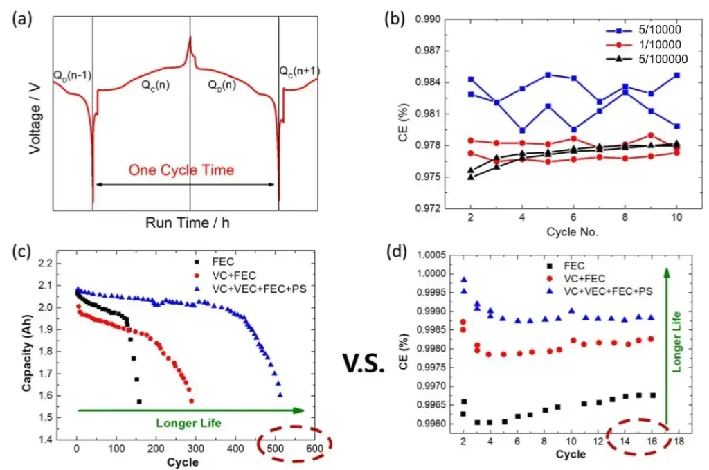
Figure 1. High-precision CE testing enables rapid battery life prediction: (a) charge-discharge curves; (b) CE test precision comparison — 1/5,000 accuracy (±0.006 fluctuation) cannot resolve electrolyte differences that require ±0.003 resolution; (c) long-cycle capacity under three electrolyte formulations; (d) early-cycle CE comparison after 16 cycles showing CE of 0.9965, 0.998, and 0.999 — a gap detectable only at 1/10,000 precision or better.

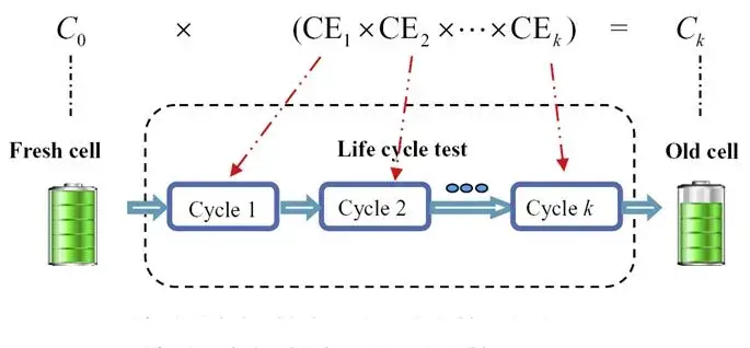
Figure 2. Coulombic Efficiency-based battery lifespan prediction model. With initial capacity C₀ = 100 Ah: at CE = 99.95%, C₅₀₀ = 77.88 Ah; at CE = 99.955%, C₅₀₀ = 79.85 Ah — a 1.97% model accuracy difference from a 0.005% CE measurement error, confirming why 0.01% test precision is required for accurate cycle life prediction.

3. Charge Endpoint Slippage (\(\Delta C\)): Internal Side Reaction Assessment

Next, let’s introduce the second significance of high-precision current & voltage testing: internal side reaction assessment of batteries. Before delving into detailed application cases, we need to introduce two concepts: Δ_C (Charge Endpoint Slippage) or Ch.End.Cap. (%). Both are derived directly from high-precision charge capacity data:

As shown in Figure 3(a), \(\Delta C\) can be calculated by subtracting the charging capacity of the previous cycle from that of the subsequent cycle, i.e., \(\Delta C = QC(n+1) – QD(n)\); while \(Ch.End.Cap.(\%)\) can be calculated by dividing the charging capacity of the \(n\)th cycle by that of the first cycle, i.e., \(Ch.End.Cap.(\%) = QC(n) / QC(1) \times 100\%\). Although these two parameters have different calculation methods, they represent the same significance, both of which can characterize the degree of oxidation reaction occurring in the electrolyte on the positive electrode side. This oxidation reaction continuously consumes the electrolyte and deposits reaction by-products on the surface of the negative electrode material. Over time, this will clog the gaps in the negative electrode material and lead to a drop in battery capacity.

The specific reaction process is illustrated in Figures 3(c) and (d). Figure 3(b) shows the charge endpoint shift of the battery under multiple cycle conditions, indicating that the positive electrode side continuously consumes active lithium in the electrolyte, gradually affecting the battery’s cycle life. Generally, in a stable cycling process, the values of Δ_C or Ch.End.Cap. (%) for mature batteries are relatively small. If the testing accuracy is too low, accurate and effective analysis results cannot be obtained. Therefore, we need high-precision testing equipment for detailed analysis of battery side reactions.

Figure 3(e) also illustrates four aspects of the application of parameters Δ_C or Ch.End.Cap. (%): ① Screening of different electrolyte additives; ② Screening of different cathode electrode materials; ③ Determination of oxidation charge under different potentials; and ④ Study of related material mechanisms.

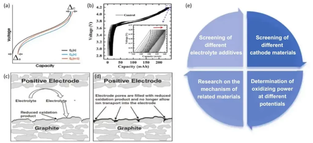
Figure 3. Charge endpoint slippage \(\Delta C\) for internal side reaction assessment: (a) definition (\(\Delta C = QC(n+1) – QD(n)\)); (b) multi-cycle endpoint shift showing ongoing cathode-side electrolyte oxidation; (c–d) oxidation reaction mechanism — electrolyte consumed at cathode, by-products deposited on anode pores; (e) four applications of \(\Delta C\) and \(Ch.End.Cap.(\%)\) in battery R&D.

Figures 4(a-c) show the comparison of cycle life of LCO batteries under three different electrolytes. Figure 4(d) extracts the Ch.End.Cap. (%) of the first 16 cycles for comparison, and it is found that the electrolytes with the addition of 1wt% or 2wt% VC have much lower Ch.End.Cap. (%) values compared to the electrolyte without VC addition.

This indicates that the addition of VC can slow down the oxidation rate of the electrolyte on the cathode electrode side, thereby extending the battery’s cycle life. From the long-term cycling results shown in Figure 4(e), it can also be seen that after cycling for 110 cycles, the capacity retention rate of the electrolyte without VC addition has dropped to around 86%, while the capacity retention rate of the electrolytes with the addition of 1wt% or 2wt% VC remains above 94%.

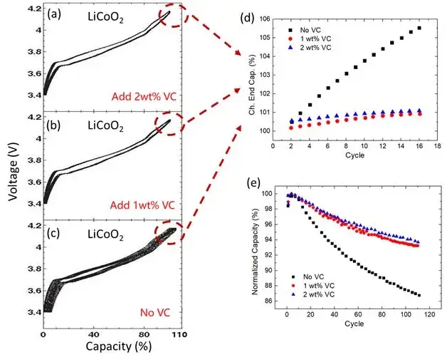
Figure 4. VC additive effect on LCO battery cycle life: (a–c) full cycle life curves; (d) Ch.End.Cap.(%) during first 16 cycles — VC-containing electrolytes show significantly lower charge endpoint slippage; (e) long-term capacity retention — without VC: 86% at 110 cycles; with 1wt% or 2wt% VC: above 94%. Early-cycle Ch.End.Cap.(%) from 16 cycles predicts 110-cycle outcome.

4. LFP dQ/dV Curve Analysis: Identifying Battery Capacity Decay Mechanisms

The dQ/dV curve (also called the incremental capacity / IC curve) and its inverse dV/dQ curve (differential voltage / DV curve) are the third class of high-precision measurement that unlocks refined battery failure analysis. These curves transform the voltage plateau regions of standard charge-discharge profiles into peaks and features that directly identify phase transitions, active material changes, and internal resistance evolution — without destructive cell teardown.

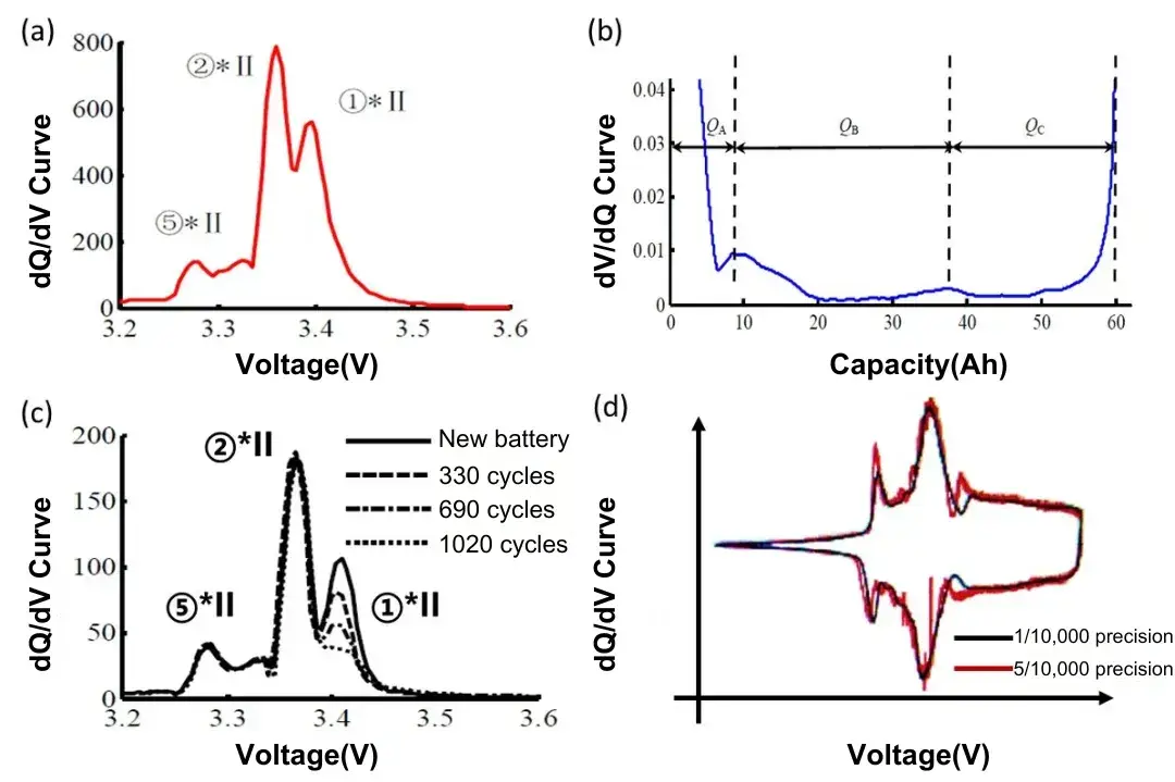
Figure 5. LFP battery dQ/dV (IC curve) and dV/dQ analysis: (a) dQ/dV curve with three phase transition peaks ⑤×II, ②×II, ①×II; (b) corresponding dV/dQ regions Q_A, Q_B, Q_C; (c) multi-cycle dQ/dV comparison — peaks ⑤×II and ②×II stable (no active material loss), peak ①×II decreases (active lithium loss, primary decay mechanism); (d) test precision comparison — 0.05% accuracy buries small phase peaks in noise; 0.01% accuracy resolves them cleanly for failure analysis.

Figure 5 illustrates three key findings from LFP dQ/dV analysis:

• Three-peak structure (Figure 5a): the LFP dQ/dV curve shows three distinct phase transition peaks (⑤×II, ②×II, ①×II) whose areas correspond to the charge capacity of each phase transition stage. The corresponding dV/dQ plot (Figure 5b) maps these to three capacity regions Q_A, Q_B, Q_C.
• Decay mechanism identification (Figure 5c): after cycling, peaks ⑤×II and ②×II remain stable in shape and area — confirming no significant active material loss. Peak ①×II decreases in height — identifying active lithium loss as the dominant capacity decay mechanism. No peak position shift means no significant internal resistance increase.
• Precision requirement (Figure 5d): at 0.05% (5/10,000) accuracy, small phase transition peaks are buried in measurement noise, making failure identification impossible. At 0.01% (1/1,000) or better accuracy, all peaks are clearly resolved — enabling detection of early-stage weak side reactions before they escalate to measurable capacity loss.

5. IEST High-Precision Electrochemical Performance Analyzer: ECT and ERT Series

The IEST ECT and ERT series Electrochemical Performance Analyzers address the requirements of all three high-precision battery analysis methods described above:

• 0.01% (1/10,000) current and voltage accuracy on all 8 channels — enabling the ±0.001 CE fluctuation required to distinguish electrolyte formulations after 16 cycles rather than 500.
• ERT7008 with integrated CV and EIS: cyclic voltammetry and electrochemical impedance spectroscopy can be inserted as steps within a long-term cycling protocol — eliminating the need to transfer cells between instruments and enabling simultaneous CE monitoring, dQ/dV analysis, and impedance tracking throughout a single cycling experiment.
• High-resolution data acquisition: the sampling density required to generate artifact-free dQ/dV and dV/dQ curves is supported natively, without requiring post-processing smoothing that can obscure genuine phase transition features.

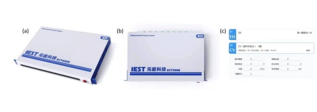
Figure 6. IEST ECT/ERT series Electrochemical Performance Analyzer: (a) ECT series high-precision cycler; (b) ERT7008 8-channel system at 0.01% accuracy; (c) integrated CV and EIS in cycling protocol — enabling simultaneous CE measurement, dQ/dV monitoring, and impedance tracking without equipment switching between instruments.

Key technical relationships established in this article:

• Coulombic Efficiency is calculated as \(CE = QD(n)/QC(n)\); a 0.005% CE measurement error produces 1.97% lifespan prediction error at 500 cycles for a 100 Ah cell.
• CE differences between electrolyte formulations of \(\leq 0.003\) (distinguishing good from poor electrolytes at 16 cycles) require test equipment precision of 0.01% or better — equipment at 0.05% accuracy cannot resolve this difference.
• LFP \(dQ/dV\) analysis identifies three phase transition peaks whose evolution across cycles separates active material loss from active lithium loss from internal resistance increase.
• \(Ch.End.Cap.(\%)\) from the first 16 cycles predicts 110-cycle capacity retention, allowing VC additive effectiveness to be confirmed in days rather than weeks.

All three analyses require the same 0.01% precision threshold, achievable with the IEST ERT7008 8-channel Electrochemical Performance Analyzer.

6. References

[1] F.F. Yang, X.B. Song, G.Z. Dong and K.L. Tsui, A coulombic efficiency-based model for prognostics and health estimation of lithium-ion batteries. Energy 171 (2019) 1173-1182.

[2] J.C. Burns, A. Kassam, N.N. Sinha, L.E. Downie, L. Solnickova, B.W. Way and J.R. Dahn, Predicting and Extending the Lifetime of Li-Ion Batteries. Journal of The Electrochemical Society 160 (2013) A1451-A1456.

[3] D.Y.H. Wang, N.N. Sinha, R. Petibon, J.C. Burns and J.R. Dahn, A systematic study of well-known electrolyte additives in LiCoO₂/graphite pouch cells. Journal of Power Sources 251 (2014) 311-318.

[4] J.C. Burns, N.N. Sinha, D.J. Coyle, G. Jain, C.M. VanElzen, W.M. Lamanna, A. Xiao, E. Scott, J.P. Gardner and J.R. Dahn, The Impact of Varying the Concentration of Vinylene Carbonate Electrolyte Additive in Wound Li-Ion Cells. Journal of The Electrochemical Society 159 (2012) A85-A90.

[5] X.B. Han,《Research on Mechanistic Model and State Estimation of Automotive Lithium-ion Batteries》, 2014.10.

7. FAQ: Coulombic Efficiency, dQ/dV Analysis, and Battery Life Prediction